Chapter 6: Simple vs. Optimal - The Power of Competition - Algorithimic Game Theory with Python

We established that the Optimal Auction (using virtual valuations and specific reserve prices) beats the Standard Second-Price auction.

However, the Optimal Auction is complex. You need detailed market data to calculate the perfect reserve price. If you get it wrong, you lose money.

The Bulow-Klemperer Theorem¶

In 1996, economists Bulow and Klemperer proved a shocking result that changed auction theory. They compared two scenarios:

The Genius: You keep $N$ bidders and run the mathematically Optimal Auction (perfect reserve price).
The Hustler: You run a simple Second-Price Auction (no reserve price), but you go out and find one extra bidder ( $N+1$ ).

The Theorem:

The Simple Auction with $N+1$ bidders earns MORE revenue than the Optimal Auction with $N$ bidders.

This teaches us a profound business lesson: It is better to invest in marketing (finding more customers) than in market research (optimizing prices). Competition is more powerful than complex math.

Strategy 2: The Single Sample¶

What if you can’t find more bidders? How do you set a reserve price without knowing the market distribution? A simple trick is the Single Sample method:

Take the first bidder’s bid.
Kick them out (sorry!).
Use their bid as the Reserve Price for everyone else.

It sounds wasteful to kick someone out, but this method is proven to get a very good approximation of the optimal revenue.

Let’s prove the Bulow-Klemperer Theorem with code.

import numpy as np
import matplotlib.pyplot as plt

def compare_auctions(num_simulations=10000):
    """
    Proves Bulow-Klemperer: 
    Simple Auction (N+1 Bidders) > Optimal Auction (N Bidders)
    """
    
    # PARAMETERS
    N = 5  # Number of bidders in the "Base" case
    # Valuation Distribution: Uniform [0, 100]
    # For U[0,100], the Optimal Reserve Price is mathematically calculated as $50.
    OPTIMAL_RESERVE = 50 
    
    rev_optimal_n = []
    rev_simple_n_plus_1 = []
    
    for _ in range(num_simulations):
        # --- SCENARIO 1: OPTIMAL AUCTION (N Bidders) ---
        # We have N bidders. We use the Perfect Reserve Price ($50).
        bids_n = np.random.uniform(0, 100, N)
        bids_n.sort() # Sort low to high
        
        # Logic:
        # 1. If highest bid < Reserve -> Revenue 0
        # 2. If highest > Reserve but 2nd highest < Reserve -> Revenue = Reserve
        # 3. If 2nd highest > Reserve -> Revenue = 2nd Highest
        
        highest = bids_n[-1]
        second = bids_n[-2]
        
        if highest < OPTIMAL_RESERVE:
            rev_optimal_n.append(0)
        elif second < OPTIMAL_RESERVE:
            rev_optimal_n.append(OPTIMAL_RESERVE)
        else:
            rev_optimal_n.append(second)
            
        # --- SCENARIO 2: SIMPLE AUCTION (N+1 Bidders) ---
        # We add 1 extra bidder. We use NO Reserve Price (Standard Vickrey).
        bids_plus = np.random.uniform(0, 100, N + 1)
        bids_plus.sort()
        
        # Revenue is simply the second highest bid
        rev_simple_n_plus_1.append(bids_plus[-2])
        
    return rev_optimal_n, rev_simple_n_plus_1

# --- RUN SIMULATION ---
rev_opt, rev_simp = compare_auctions()

avg_opt = np.mean(rev_opt)
avg_simp = np.mean(rev_simp)

print(f"--- The Bulow-Klemperer Theorem ---")
print(f"Scenario 1: Optimal Auction (Complex) with N Bidders")
print(f"Average Revenue: ${avg_opt:.2f}")
print(f"\nScenario 2: Simple Auction (Vickrey) with N+1 Bidders")
print(f"Average Revenue: ${avg_simp:.2f}")

diff = avg_simp - avg_opt
print(f"\nResult: Simply adding 1 bidder beat the optimal math by ${diff:.2f} per auction!")

# --- VISUALIZATION ---
plt.figure(figsize=(10, 6))
plt.hist(rev_opt, bins=30, alpha=0.5, label=f'Optimal (N Bidders)', color='red')
plt.hist(rev_simp, bins=30, alpha=0.5, label=f'Simple (N+1 Bidders)', color='blue')
plt.axvline(avg_opt, color='red', linestyle='--', linewidth=2)
plt.axvline(avg_simp, color='blue', linestyle='--', linewidth=2)
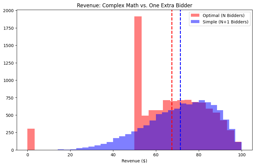
plt.title("Revenue: Complex Math vs. One Extra Bidder")
plt.xlabel("Revenue ($)")
plt.legend()
plt.show()

--- The Bulow-Klemperer Theorem ---
Scenario 1: Optimal Auction (Complex) with N Bidders
Average Revenue: $67.32

Scenario 2: Simple Auction (Vickrey) with N+1 Bidders
Average Revenue: $71.31

Result: Simply adding 1 bidder beat the optimal math by $3.98 per auction!

Analysis¶

The simulation confirms the Bulow-Klemperer Theorem.

Even though Scenario 1 used the perfect mathematical reserve price (derived from Myerson’s Lemma), it couldn’t beat Scenario 2, which used no math at all but had just one extra participant.

Key Takeaways for Mechanism Design:

Market Thickness matters more than Market Design. If you can get more people to show up, you don’t need complex rules.
Robustness. The Simple Auction works for any distribution. The Optimal Auction fails if you guessed the distribution wrong (e.g., if you thought the reserve should be $50 but the market changed and it should be $30).
Simplicity. Simple auctions (like eBay’s) are often preferred not just because they are easy to code, but because they are “Prior-Independent.” They work well without knowing secret information about the bidders.