Chapter 13: Potential Games - The Physics of Game Theory - Algorithimic Game Theory with Python

A major fear in Game Theory is Chaos. If players keep changing their minds to get a better deal, will they cycle forever?

The Problem of Existence¶

In many games (like Rock-Paper-Scissors), there is no stable state (Pure Nash Equilibrium). However, Congestion Games (like Traffic Routing) are special.

Rosenthal’s Theorem (1973)¶

Rosenthal proved that in any congestion game, a Pure Nash Equilibrium always exists. He did this by discovering a “Magic Number” called the Potential Function ( $\Phi$ ).

The Physics Analogy¶

Think of a ball rolling on a hilly terrain.

Gravity pulls it down (Minimizing Potential Energy).
Eventually, the ball must stop at the bottom of a valley.

Rosenthal showed that Selfish Drivers are like that ball. Every time a driver switches roads to save time (a “Better Response”), they mathematically lower the Potential Function of the system. Since the potential cannot drop below zero, the system must stop eventually. When it stops, we are at a Nash Equilibrium.

The “Magic” Potential Function¶

The potential is not the Total Travel Time (Social Cost). It is slightly different:

\Phi = \sum_{e \in \text{Roads}} \sum_{i=1}^{k} c_e(i)

(1)

Where $c_e(i)$ is the cost of the road when $i$ people are on it.

Let’s simulate this “Gravity” by running Best-Response Dynamics.

import random
import matplotlib.pyplot as plt

def solve_potential_game():
    """
    Simulates Best-Response Dynamics in a Congestion Game.
    Demonstrates that the 'Potential Function' always decreases, ensuring convergence.
    """
    
    # --- SETUP ---
    # 50 Drivers, 3 Roads
    NUM_DRIVERS = 50
    ROADS = ['A', 'B', 'C']
    
    # Cost Functions (Congestion)
    # Road A: Very steep (gets slow fast) -> Cost = 3 * count
    # Road B: Medium -> Cost = 2 * count + 10
    # Road C: Flat but long -> Cost = 1 * count + 50
    def get_cost(road, num_cars):
        if road == 'A': return 3 * num_cars
        if road == 'B': return 2 * num_cars + 10
        if road == 'C': return 1 * num_cars + 50
        return 9999

    # Rosenthal's Potential Function
    # Phi = Sum over roads of (Sum_{i=1 to k} Cost(i))
    def calculate_potential(current_allocation):
        phi = 0
        counts = {r: 0 for r in ROADS}
        for d in current_allocation:
            counts[d] += 1
            
        for r in ROADS:
            k = counts[r]
            # Sum of costs for the 1st car, 2nd car, ... kth car
            for i in range(1, k + 1):
                phi += get_cost(r, i)
        return phi

    # Initial State: Random allocation
    allocation = [random.choice(ROADS) for _ in range(NUM_DRIVERS)]
    
    potential_history = []
    
    print(f"--- Starting Best-Response Dynamics ---")
    
    # --- ITERATION LOOP ---
    # In each step, pick a random driver and see if they want to move.
    converged = False
    step = 0
    max_steps = 1000
    
    while not converged and step < max_steps:
        step += 1
        current_potential = calculate_potential(allocation)
        potential_history.append(current_potential)
        
        # Pick a random driver
        driver_idx = random.randint(0, NUM_DRIVERS - 1)
        current_road = allocation[driver_idx]
        
        # Calculate current counts
        counts = {'A': 0, 'B': 0, 'C': 0}
        for r in allocation: counts[r] += 1
        
        # Cost I am paying now
        my_current_cost = get_cost(current_road, counts[current_road])
        
        # Check other roads
        best_road = current_road
        best_cost = my_current_cost
        
        for alt_road in ROADS:
            if alt_road == current_road: continue
            
            # If I switch, count on alt_road increases by 1
            new_cost = get_cost(alt_road, counts[alt_road] + 1)
            
            if new_cost < best_cost:
                best_road = alt_road
                best_cost = new_cost
        
        # MOVE!
        if best_road != current_road:
            allocation[driver_idx] = best_road
            # Note: We don't print every move to keep output clean
        else:
            # If this driver is happy, check if EVERYONE is happy
            # (In a real full simulation, we'd need to check all drivers to confirm Nash)
            pass
            
        # Check for Convergence (No moves for many steps)
        # Simplified: If potential hasn't changed in 50 steps, we assume convergence
        if step > 50 and potential_history[-1] == potential_history[-50]:
            converged = True

    # --- RESULTS ---
    print(f"Converged in {step} steps.")
    print(f"Final Potential: {potential_history[-1]}")
    
    # Count final allocation
    final_counts = {'A': 0, 'B': 0, 'C': 0}
    for r in allocation: final_counts[r] += 1
    print(f"Final Counts: {final_counts}")
    print(f"Final Costs: A={get_cost('A', final_counts['A'])}, B={get_cost('B', final_counts['B'])}, C={get_cost('C', final_counts['C'])}")

    # --- VISUALIZATION ---
    plt.figure(figsize=(10, 6))
    plt.plot(potential_history, linewidth=2, color='purple')
    plt.title("Rosenthal's Potential Function Over Time")
    plt.xlabel("Simulation Steps (Driver Updates)")
    plt.ylabel("Potential Value (Phi)")
    plt.grid(True, alpha=0.3)
    plt.show()

solve_potential_game()

--- Starting Best-Response Dynamics ---
Converged in 72 steps.
Final Potential: 1788
Final Counts: {'A': 19, 'B': 23, 'C': 8}
Final Costs: A=57, B=56, C=58

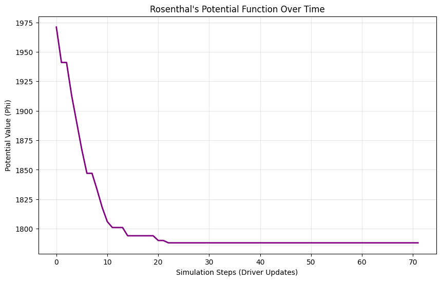
Analysis: The Descent to Equilibrium¶

Look at the graph produced by the code.

Strictly Decreasing: Notice that the curve never goes up.
Convergence: It eventually flattens out. This flat line is the Pure Nash Equilibrium.

Why does this matter? This proves that complex distributed systems (like the Internet routing protocols BGP or TCP) can be stable even without a central dictator. As long as the game has the structure of a “Potential Game,” we don’t need to worry about infinite loops or chaos. The “Physics” of the game guarantees stability.