Chapter 5: Revenue Maximization - The Art of the Reserve Price

Until now, we have been “benevolent” designers. We wanted the item to go to the highest bidder ( $v_i$ ) to maximize societal happiness.

But what if you are a seller (like Google or a government selling spectrum)? You care about Revenue.

The Conflict: Welfare vs. Revenue¶

Imagine a single bidder, Alice, with a valuation $v \sim U[0, 100]$ (Uniformly distributed).

Welfare Maximizer: We just give it to her (price $0). She is happy ( $v$ ), we get $0. Total Welfare = $v$ .
Revenue Maximizer: We set a price tag (Take-it-or-leave-it).
- If we set price $10: She buys often, but we make little.
- If we set price $90: We make a lot per sale, but she rarely buys.

This is the classic Monopoly Pricing Problem.

The Solution: Myerson’s Optimal Auction¶

Roger Myerson (yes, him again) proved that to maximize revenue, we shouldn’t look at the bids directly. We should look at the Virtual Valuations ( $\phi$ ).

The “Virtual Valuation” is a formula that adjusts a bid based on the probability distribution of the bidder’s value.

\phi(v_i) = v_i - \frac{1 - F(v_i)}{f(v_i)}

(1)

$v_i$ : The bid.
$F(v_i)$ : The probability someone has a value less than this (CDF).
$f(v_i)$ : The probability density (PDF).

The Optimal Auction Rule:

Calculate $\phi(v_i)$ for everyone.
Winner is the person with the highest Virtual Valuation (provided $\phi > 0$ ).
The point where $\phi(v) = 0$ acts as the Optimal Reserve Price.

Let’s simulate this for a Uniform Distribution (where the math is easy).

import numpy as np
import matplotlib.pyplot as plt

def run_revenue_simulation(num_auctions=10000):
    """
    Compares Standard Second-Price Auction vs. Optimal Auction (with Reserve)
    Scenario: 2 Bidders, Valuations drawn from Uniform [0, 100]
    """
    
    # 1. Setup
    # Uniform Distribution U[0, 100]
    # For U[0,100], the Virtual Valuation is phi(v) = 2v - 100.
    # We want phi(v) >= 0, so 2v >= 100 --> v >= 50.
    # Therefore, the Optimal Reserve Price is $50.
    RESERVE_PRICE = 50 
    
    revenue_standard = []
    revenue_optimal = []
    
    for _ in range(num_auctions):
        # Generate random values for Bidder A and Bidder B
        bids = np.random.uniform(0, 100, 2)
        bids.sort() # Sort so bids[0] is low, bids[1] is high
        
        low_bid = bids[0]
        high_bid = bids[1]
        
        # --- MECHANISM A: STANDARD VICKREY (Second Price) ---
        # Highest bidder wins, pays second highest price.
        # Reserve is effectively $0.
        revenue_standard.append(low_bid)
        
        # --- MECHANISM B: MYERSON OPTIMAL (Reserve Price $50) ---
        # Rule: Both must bid at least $50.
        
        # Case 1: Both fail reserve (Both < 50) -> No Sale
        if high_bid < RESERVE_PRICE:
            revenue_optimal.append(0)
            
        # Case 2: Only one clears reserve (High > 50, Low < 50) -> Pay Reserve
        elif high_bid >= RESERVE_PRICE and low_bid < RESERVE_PRICE:
            revenue_optimal.append(RESERVE_PRICE)
            
        # Case 3: Both clear reserve -> Pay Second Highest (Standard)
        else: # Both >= 50
            revenue_optimal.append(low_bid)
            
    return revenue_standard, revenue_optimal

# Run Simulation
rev_std, rev_opt = run_revenue_simulation()

# --- ANALYSIS ---
avg_std = np.mean(rev_std)
avg_opt = np.mean(rev_opt)
lift = ((avg_opt - avg_std) / avg_std) * 100

print(f"--- Revenue Comparison (2 Bidders, U[0,100]) ---")
print(f"Average Revenue (Standard 2nd Price): ${avg_std:.2f}")
print(f"Average Revenue (Optimal /w Reserve): ${avg_opt:.2f}")
print(f"Revenue Increase: +{lift:.1f}%")

# --- VISUALIZATION ---
plt.figure(figsize=(10,5))
plt.hist(rev_std, bins=50, alpha=0.5, label='Standard Revenue', color='blue')
plt.hist(rev_opt, bins=50, alpha=0.5, label='Optimal Revenue', color='green')
plt.axvline(avg_std, color='blue', linestyle='dashed', linewidth=2)
plt.axvline(avg_opt, color='green', linestyle='dashed', linewidth=2)
plt.title(f"Impact of Reserve Price ($50) on Seller Revenue")
plt.xlabel("Revenue per Auction ($)")
plt.ylabel("Frequency")
plt.legend()
plt.show()

--- Revenue Comparison (2 Bidders, U[0,100]) ---
Average Revenue (Standard 2nd Price): $33.52
Average Revenue (Optimal /w Reserve): $41.64
Revenue Increase: +24.2%

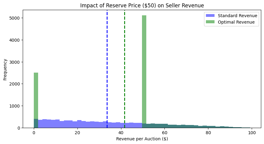
What just happened?¶

You should see that the Optimal Auction generated significantly more revenue (usually around 10-15% more in this specific setting).

How did it do that? Look at the histogram or the logic in the code:

The “Standard” Auction often sells for very low prices (e.g., if bids are $5 and $2, revenue is $2).
The “Optimal” Auction refuses to sell for less than $50.
- If the high bidder was $80 and the low bidder was $2, the price jumps from $2 to $50 (the reserve).
- Trade-off: Sometimes nobody buys (if both are < $50), so we get $0.

Conclusion: By risking a “no-sale,” the seller forces high-value bidders to pay a premium. This demonstrates that Market Efficiency (Social Welfare) and Profit (Revenue) are often at odds. To make the most money, you sometimes have to refuse to sell to people who want the item!