Chapter 1: Introduction - When Selfish is Slow
Welcome to Algorithmic Game Theory! In this book, we explore what happens when computer science meets economics. We aren’t just looking at algorithms that run on a single computer; we are looking at systems where the “inputs” are people (or agents) who are trying to maximize their own benefit.
The Core Concept: The Price of Anarchy
One of the biggest surprises in this field is that selfish behavior can hurt everyone, including the people being selfish. We often assume that giving people more options (like building a new road) will always improve the situation. Game Theory shows us this isn’t true.
This phenomenon is captured by Braess’s Paradox.
The Scenario
Imagine 4,000 drivers want to get from a Start point to an End point.
There are two initial routes: Top and Bottom.
Each route has two parts: a wide highway (fast, always takes 45 mins) and a narrow road (slow, takes longer if there is traffic).
The Paradox: If we build a super-fast “teleport” road connecting the middle points, everyone will try to use it to save time. But because everyone does this, the traffic jams get so bad that every single driver arrives later than before.
This proves that individual rationality (doing what is best for you) can lead to collective irrationality (a result that is bad for everyone).
import networkx as nx
import matplotlib.pyplot as plt

def draw_braess_network():
    # 1. Create a directed graph
    G = nx.DiGraph()

    # 2. Add Nodes
    # Positions: Start (Left), End (Right), A (Top), B (Bottom)
    pos = {
        'Start': (0, 1),
        'End': (2, 1),
        'A': (1, 2),
        'B': (1, 0)
    }

    # 3. Add Edges (Roads) with labels for their Cost (Travel Time)
    # T = number of cars
    edges = [
        ('Start', 'A', 'Narrow\n(T / 100)'),
        ('Start', 'B', 'Wide\n(45 mins)'),
        ('A', 'End', 'Wide\n(45 mins)'),
        ('B', 'End', 'Narrow\n(T / 100)'),
        # The Shortcut
        ('A', 'B', 'Shortcut\n(0 mins)')
    ]

    G.add_edges_from([(u, v) for u, v, label in edges])

    # 4. Draw the Graph
    plt.figure(figsize=(10, 6))

    # Draw Nodes
    nx.draw_networkx_nodes(G, pos, node_size=2000, node_color='lightblue', edgecolors='black')
    nx.draw_networkx_labels(G, pos, font_size=12, font_weight='bold')

    # Draw Edges
    nx.draw_networkx_edges(G, pos, arrowstyle='->', arrowsize=20, edge_color='gray', width=2)

    # Draw Edge Labels (The Costs)
    edge_labels = {(u, v): label for u, v, label in edges}
    nx.draw_networkx_edge_labels(G, pos, edge_labels=edge_labels, font_color='red', font_size=10)

    # Title and Layout
    plt.title("The Braess's Paradox Network", fontsize=15)
    plt.axis('off') # Turn off the x/y axis numbers
    plt.margins(0.2)
    plt.show()

# Run the function to display the graph
draw_braess_network()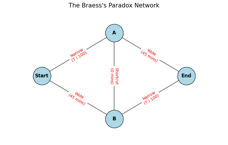
import matplotlib.pyplot as plt

def calculate_travel_time(drivers, use_shortcut=False):
    """
    Calculates total travel time for a single driver based on traffic distribution.

    Path options:
    1. Start -> A -> End (Top Path)
    2. Start -> B -> End (Bottom Path)
    3. Start -> A -> B -> End (The Zig-Zag Shortcut)
    """

    # Cost functions
    # Wide road: Always takes 45 minutes
    # Narrow road: Takes (number_of_drivers / 100) minutes

    if not use_shortcut:
        # NASH EQUILIBRIUM WITHOUT SHORTCUT
        # Drivers split 50/50 because paths are identical.
        drivers_top = drivers / 2
        drivers_bottom = drivers / 2

        # Time = (Narrow Road) + (Wide Road)
        time_top = (drivers_top / 100) + 45
        time_bottom = 45 + (drivers_bottom / 100)

        return time_top

    else:
        # NASH EQUILIBRIUM WITH SHORTCUT
        # The shortcut (A->B) is instantaneous (0 mins).
        # Everyone tries to take Start->A->B->End because A is better than the wide road
        # and B is better than the wide road.

        # All 4000 drivers jam into the narrow roads.
        time_zigzag = (drivers / 100) + 0 + (drivers / 100)
        return time_zigzag

# --- Parameters ---
total_drivers = 4000

# 1. Calculate Time WITHOUT the shortcut
time_before = calculate_travel_time(total_drivers, use_shortcut=False)

# 2. Calculate Time WITH the shortcut
time_after = calculate_travel_time(total_drivers, use_shortcut=True)

# --- Output Results ---
print(f"--- Braess's Paradox Simulation ---")
print(f"Total Drivers: {total_drivers}")
print(f"\nScenario 1: Two separate routes (No shortcut)")
print(f"Travel Time per Driver: {time_before} minutes")

print(f"\nScenario 2: Ultra-fast shortcut added")
print(f"Travel Time per Driver: {time_after} minutes")

print(f"\nResult: Adding the shortcut made everyone {time_after - time_before} minutes slower!")

# --- Visualization ---
labels = ['Before Shortcut', 'After Shortcut']
times = [time_before, time_after]

plt.figure(figsize=(8, 5))
plt.bar(labels, times, color=['green', 'red'])
plt.ylabel('Minutes to Commute')
plt.title("Impact of 'Selfish Routing' on Travel Time")
plt.ylim(0, 90)
for i, v in enumerate(times):
    plt.text(i, v + 2, str(v) + " mins", ha='center', fontweight='bold')
plt.show()
--- Braess's Paradox Simulation ---
Total Drivers: 4000
Scenario 1: Two separate routes (No shortcut)
Travel Time per Driver: 65.0 minutes
Scenario 2: Ultra-fast shortcut added
Travel Time per Driver: 80.0 minutes
Result: Adding the shortcut made everyone 15.0 minutes slower!
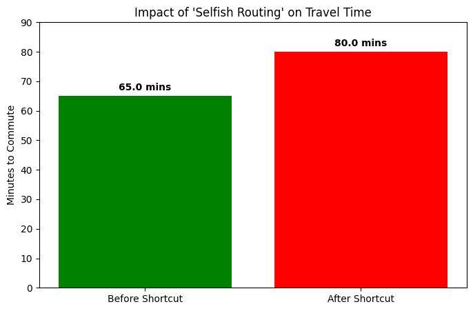
What just happened?
In the code above, you will see that adding a shortcut (Scenario 2) actually increased travel time from 65 minutes to 80 minutes.
Before: Drivers split up. Traffic was balanced.
After: The “Narrow” roads became so attractive individually that everyone used them, causing a massive bottleneck.
This teaches us that simply “adding capacity” (like building more roads or buying more servers) doesn’t always solve congestion if you ignore game theory!